
Explaining Linear Models with Categorical Features
Published:
This fifth blog post demonstrates how Linear Models can be adapted to work with Categorical Feature, that is, features that are not naturally represented with numbers. Machine Learning models require numerical input features to work properly and so one Categorical Features must be preprocessed. While One-Hot-Encoding is the go-to practice when a linear model is used downstream, the interpretation of the resulting model coefficients is not trivial. We advocate viewing linear models fitted on One-Hot-Encoded features as a particular instance of Parametric Additive Models, which we know how to explain faithfully.
Categorical Features
The objective of supervised learning is to accurately predict a target \(y\) given an input \(x\). The input components \(x_i\) (or features) are generally assumed to be numerical e.g. \(x_i=1.6223\). In fact, this is a crucial assumption for linear models
\[h(x) = \omega_0 + \sum_{i=1}^d \omega_i x_i.\]If \(x_i\) is not numerical, the expression \(\omega_i x_i\) does not make much sense! Nevertheless, many datasets involves features that are non-numerical, which we will call categorical for simplicity. For example, in the Mushroom dataset from the UCI repository, each instance \(x\) represents a different specie of mushroom and categorical features \(x_i\) are used to characterize said mushrooms. The label \(y\) to predict is whether the mushroom is edible \(y=0\) or poisonous \(y=1\).
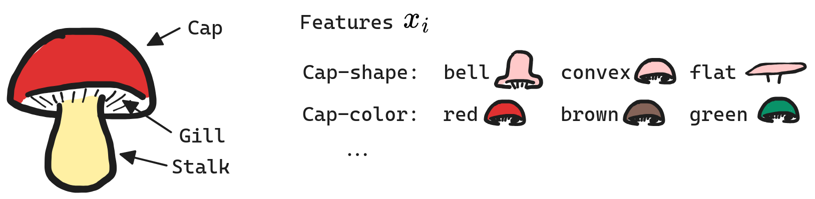
These features are not easily translated into numbers. For example, the values red, brown, and green for the feature cap-color could be given the numerical values \(1\), \(2\), and \(3\). However, doing so imposes an arbitrary ordering between the categories. Why should the color green be given a larger value than color red? The performance of the linear model used downstream will be highly sensitive to our choice of ordering, so we must look for a better alternative.
The common solution is to first assign arbitrary numbers to the categories, and then use a One-Hot-Encoder. Assuming feature \(x_i\) can take \(C\) different values, a One-Hot-Encoder represents the feature \(x_i\) using a vector of \(C\) components. The specific instance \(x_i=c\) is encoded as the vector whose components are all zero, except for the \(c^\text{th}\), whose value is \(1\).
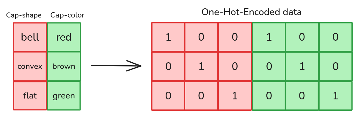
This data preprocessing allows the model to distinguish the different categories without imposing a specific order between them. One-Hot-Encoding works especially well for linear models, in fact, it allows us to reach perfect test accuracy on the Mushroom dataset.
import numpy as np
from pyfd.data import get_data_mushroom
from sklearn.model_selection import train_test_split
from sklearn.linear_model import LogisticRegression
from sklearn.preprocessing import OneHotEncoder

X, y, features = get_data_mushroom()
print(X.shape)
>>> (8124, 21)
ohe = OneHotEncoder()
# We fit the OHE using the whole dataset. There is no data leakage since the encoder
# does not see the labels. We do this to avoid issues where the test set contains
# categories that were not seen during training.
ohe.fit_transform(X)
X_encoded = ohe.transform(X)
print(X_encoded.shape)
>>>(8124, 116)
X_train, X_test, y_train, y_test = train_test_split(X_encoded, y, test_size=0.2, random_state=42)
model = LogisticRegression(max_iter=1000, random_state=42)
model.fit(X_train, y_train)
print(model.score(X_test, y_test))
>>> 1.0
Interpretting the Model
Looking at all Coefficients
So far so good. We were able to fit an accurate linear model by carefully preprocessing the data before feading it to the model. But how should we interpret the resulting model? It is a common practice to report the weights \(\omega_i\) in order to get some overview of the model’s inner working. For instance, this scheme is presented in a tutorial of the Scikit-Learn Python library Here.
Let’s look at the result for the Mushroom prediction use-case.
coefficient cap-shape-conical : 0.38
coefficient cap-shape-convex : 0.47
coefficient cap-shape-flat : -0.14
coefficient cap-shape-knobbed : -0.06
coefficient cap-shape-sunken : 0.01
coefficient cap-surface-grooves : -0.60
coefficient cap-surface-scaly : -0.82
coefficient cap-surface-smooth : 0.63
coefficient cap-color-buff : -0.03
coefficient cap-color-cinnamon : 0.28
coefficient cap-color-gray : -0.30
coefficient cap-color-green : 0.98
coefficient cap-color-pink : -1.06
coefficient cap-color-purple : 0.10
coefficient cap-color-red : -0.40
coefficient cap-color-white : 0.83
coefficient cap-color-yellow : -0.45
coefficient bruises-no : 0.08
coefficient odor-anise : 0.53
coefficient odor-creosote : -0.25
coefficient odor-fishy : 0.07
coefficient odor-foul : -0.01
coefficient odor-musty : -2.63
coefficient odor-none : -2.64
coefficient odor-pungent : 2.56
coefficient odor-spicy : 0.78
coefficient gill-attachment-free : 2.77
coefficient gill-spacing-crowded : 0.34
coefficient gill-size-narrow : -3.96
coefficient gill-color-brown : 2.07
coefficient gill-color-buff : 0.78
coefficient gill-color-chocolate : -0.11
coefficient gill-color-gray : 0.17
coefficient gill-color-green : 1.64
coefficient gill-color-orange : -1.58
coefficient gill-color-pink : -2.22
coefficient gill-color-purple : 2.29
coefficient gill-color-red : -0.47
coefficient gill-color-white : -0.63
coefficient gill-color-yellow : 1.89
coefficient stalk-shape-tapering : 0.09
coefficient stalk-root-club : -0.03
coefficient stalk-root-equal : 0.66
coefficient stalk-root-missing : -0.10
coefficient stalk-root-rooted : -0.53
coefficient stalk-surface-above-ring-scaly : -0.17
coefficient stalk-surface-above-ring-silky : -0.53
coefficient stalk-surface-above-ring-smooth : -0.38
coefficient stalk-surface-below-ring-scaly : 0.28
coefficient stalk-surface-below-ring-silky : 0.71
coefficient stalk-surface-below-ring-smooth : -0.64
coefficient stalk-color-above-ring-buff : 2.49
coefficient stalk-color-above-ring-cinnamon : -1.09
coefficient stalk-color-above-ring-gray : 0.00
coefficient stalk-color-above-ring-orange : -0.62
coefficient stalk-color-above-ring-pink : -0.71
coefficient stalk-color-above-ring-red : -0.82
coefficient stalk-color-above-ring-white : 0.13
coefficient stalk-color-above-ring-yellow : 1.90
coefficient stalk-color-below-ring-buff : -1.15
coefficient stalk-color-below-ring-cinnamon : -1.16
coefficient stalk-color-below-ring-gray : 1.24
coefficient stalk-color-below-ring-orange : 0.47
coefficient stalk-color-below-ring-pink : -0.48
coefficient stalk-color-below-ring-red : -0.23
coefficient stalk-color-below-ring-white : 0.24
coefficient stalk-color-below-ring-yellow : 0.34
coefficient veil-color-orange : -0.37
coefficient veil-color-white : -0.30
coefficient veil-color-yellow : 0.26
coefficient ring-number-one : -0.53
coefficient ring-number-two : 0.05
coefficient ring-type-flaring : 0.62
coefficient ring-type-large : -1.08
coefficient ring-type-none : 0.23
coefficient ring-type-pendant : 0.34
coefficient spore-print-color-brown : -0.34
coefficient spore-print-color-buff : -0.30
coefficient spore-print-color-chocolate : 0.44
coefficient spore-print-color-green : -0.41
coefficient spore-print-color-orange : 0.34
coefficient spore-print-color-purple : 0.85
coefficient spore-print-color-white : -0.16
coefficient spore-print-color-yellow : -0.14
coefficient population-clustered : -0.25
coefficient population-numerous : 0.62
coefficient population-scattered : 0.34
coefficient population-several : -0.07
coefficient population-solitary : -0.20
coefficient habitat-leaves : 0.60
coefficient habitat-meadows : -1.45
coefficient habitat-paths : 0.72
coefficient habitat-urban : 0.34
coefficient habitat-waste : -0.14
coefficient habitat-woods : -1.31
That is a lot of coefficients to report and interpret! I couln’t bother looking at each individual one to understand how my model works.
Correctly Explaining the Model
It would be better to report a single importance score per feature \(x_i\), instead of a separate coefficient for each category of each feature. To do so, we must rewrite the linear model in a different form. Letting \(\mathbf{1}(\cdot)\) be an indicator function
\[\mathbf{1}(\text{statement})= \begin{cases} 1 & \text{if statement is true}\\ 0 & \text{otherwise} \end{cases}\]a linear model fitted on one-hot-encoded features can be written
\[h(x) = \omega_0 + \omega_1 \mathbf{1}(x_1=a) + \omega_2 \mathbf{1}(x_1=b) + \omega_3 \mathbf{1}(x_2=c) + \omega_4 \mathbf{1}(x_2=d) + \omega_5 \mathbf{1}(x_2=e) + \ldots\]This is nothing more than a Parametric Additive model in disguise
\[h(x) = \omega_0 + h_1(x_1) + h_2(x_2) + \ldots\]where the basis functions along feature \(x_i\) are the Indicators \(\mathbf{1}(x_i=c)\) for the different categories that \(x_i\) can take. Remember that a previous blog post presented how to interpret Parametric Additive Models. The key idea was to fix a reference distribution \(\mathcal{B}\) and explain the Gap between the average prediction over \(\mathcal{B}\) and the prediction \(h(x)\) by reporting
\[\text{Importance of feature } i = h_i(x_i) - \mathbb{E}_{z\sim\mathcal{B}}[h_i(z_i)]\]This principle still applies altough here and so we use PyFD to compute feature importance scores.
from pyfd.decompositions import get_components_linear
from pyfd.plots import partial_dependence_plot, bar

foreground = X
background = X
# We use the get_components_linear like in previous tutorials on linear models
decomp = get_components_linear(model, foreground, background, features)
partial_dependence_plot(decomp, foreground, features)
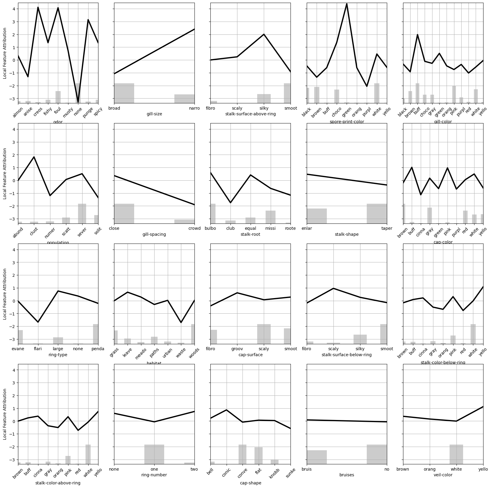
This plot illustrates the local importance of each feature. The higher the local importance (more positive) the more a specific mushroom characteristic increases the risk of being poisonous relative to the average mushroom. Although this visualization is more helpful than reporting the coefficients of the linear model, I still think it is too verbose because of the large number of features.
To adress this issue, we can compute global feature importance scores
\[\text{Global Importance of } i = \sqrt{\mathbb{E}[(\text{Local Importance of } x_i)^2]}\]GFI = np.stack([(decomp[(i,)]**2).mean() for i in range(len(features))])
GFI = np.sqrt(GFI)
features_names = features.names()
bar(GFI, features_names)
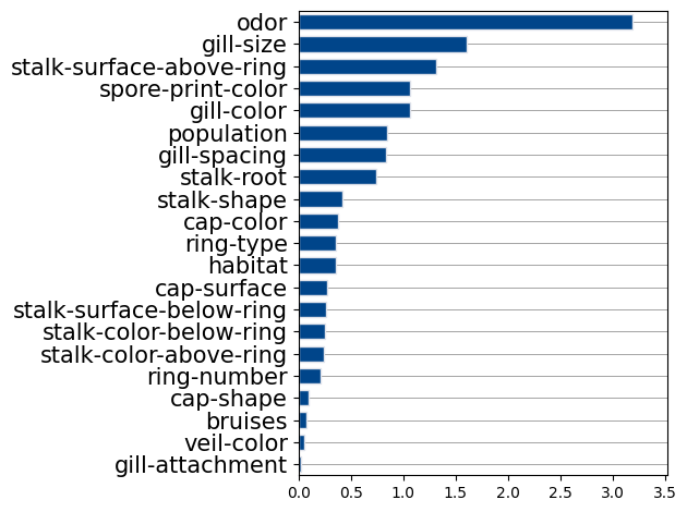
This plot shows which features are most used by the model globally. I found that keeping the five most important features and retraining the model on them led to identical test performance. We can rerun get_components_linear on this new reduced model to discover the following trends.
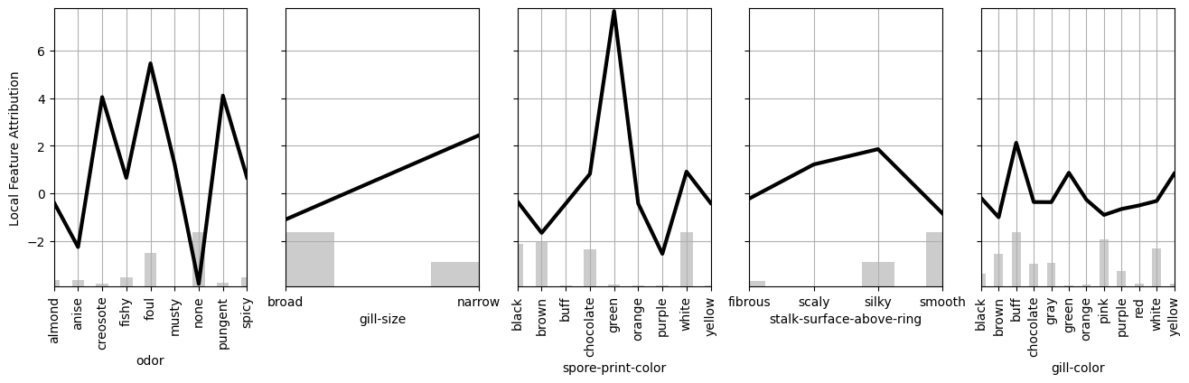
Here are the main takeaways from this figure.
- Do not consume mushrooms that have a creosote, foul, or pungent
odor. - Avoid mushrooms with a narrow
gill-size. - Never eat mushrooms with a green
spore-print-color.
Ouverture
If your data involves categorical features and you wish to use a linear model, then your first reflex should be to one-hot-encode your features. After doing so however, you might have a hard time interpreting all the coefficients of the linear model. In that case, I advocate viewing the linear model as a Parametric Additie Model fitted with Indicator basis functions \(\mathbf{1}(\cdot)\). Then, PyFD can then be used to interpret the model like we would any other additive model. Doing so provides a distinct importance score per feature, instead of each category of each feature. These less verbose explanations are useful for feature selection and understanding the model behavior locally.