Explaining Linear Models

In this second blog post, we will introduce linear models and how to interpret/explain their predictions. Although such models are rarely the most performant, understanding how to explain them is the first step toward explaining more complex models.

Linear Models

Linear Models are functions that take the following form

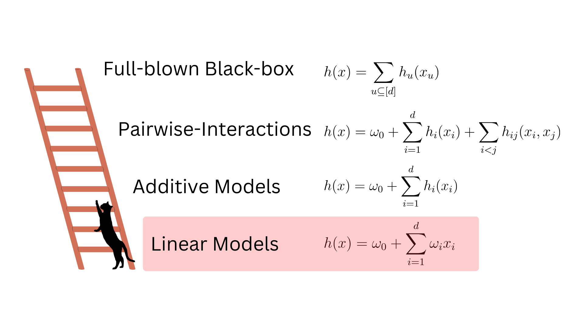
where the parameter \(\omega_0\) is called the intercept and \(\omega_1, \omega_2, \ldots, \omega_d\) are called the weights. These models are considered highly interpretable for two reasons:

1. The effect of varying feature \(x_i\) on the response \(h(x)\) is independent of the fixed values of the remaining features \(x_1, \ldots, x_{i-1}, x_{i+1}, \ldots, x_d\).
2. The effect of varying feature \(x_i\) on the response \(h(x)\) is entirely encoded in the corresponding weight \(\omega_i\).

These properties imply that, when you know the weight \(\omega_i\), you know exactly how feature \(x_i\) impacts the model output. For instance, if you have \(\omega_i=2.5\), then you know that increasing \(x_i\) by \(1\) will systematically increase the model output by \(2.5\), regardless of the value of any other features and the value of \(x_i\) itself.

As such, Linear Models are not considered black-boxes because you can simulate them in your head (assuming the number of weights \(d\) is not too large). Yet, the main objective of my research is to explain black-boxes. So why should we care about linear models?

As we shall see, explaining Linear Models predictions is not trivial and requires introducing definitions that will be useful when generalizing to black-box models.

Visually, you can see Linear Models as the first floor of the ladder we must climb before being able to explain general black-boxes.

Naively Explaining Linear Models

Imagine using a Linear Model to predict the risk that a bank applicant will default on their loan. Assuming the model \(h(x)\) returns a high-risk, the applicant \(x\) might be entitled to know which characteristics \(x_i\) led to said risk. That person would be reassured to know that the prediction was impacted by factor under their control (credit-score, salary, etc.) and not on more sensitive information (location, age, race). But how do you explain the importance of feature \(x_i\) toward a specific prediction \(h(x)\)? It is tempting to use the following definition

This makes sense apriori given that the term \(\omega_i x_i\) is exactly the component of the function that involves the feature \(i\). To understand the issue with this formulation however, we must study a very simple example involving a single feature.

import numpy as np
import matplotlib.pyplot as plt
from sklearn.linear_model import LinearRegression
np.random.seed(42)

# One feature
X = np.random.uniform(1, 2, size=(100, 1))
# The target is a simple linear function of x
y = 2 - X.ravel() + 0.1 * np.random.normal(size=(100,))
model = LinearRegression().fit(X, y)
# A point of interest to explain
x_explain = np.array([1.1])
pred = model.intercept_ + model.coef_[0]*x_explain

In this example, we have a single feature \(x\) and the target is a simple linear function \(y=2-x+\epsilon\), where \(\epsilon\) is random Gaussian noise. We can plot the data along side the model predictions.

plt.figure()
# Data
plt.scatter(X.ravel(), y)
plt.vlines(0, 0, 2.2, 'k', linewidth=1)
# Model predictions
line = np.linspace(-2, 2, 10)
plt.plot(line, model.intercept_ + model.coef_[0]*line, 'k-', linewidth=4)
# Point to explain
plt.scatter(x_explain, pred, marker="*", c='r', s=200, zorder=3)
# The local importance at x_explain
plt.plot([0, x_explain, x_explain], [model.intercept_, model.intercept_, pred], 'k--', linewidth=2)
plt.text(x_explain+0.07, (model.intercept_ +  pred) / 2, r"$\omega x_{\text{explain}}$")
plt.xlim(-0.2, 2)
plt.ylim(0, 2.2)
plt.xlabel("x")
plt.ylabel("y")

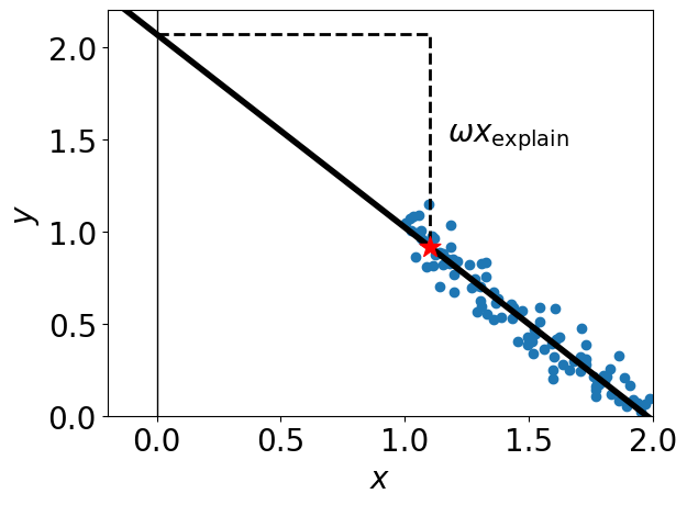
Here, the blue points are the data, the thick black line is the model prediction \(h(x)\) on all \(x\) values, and the red star is the point of interest \(x_{\text{explain}}\) along with the prediction \(h(x_{\text{explain}})\). Assuming the target \(y\) represents the risk of defaulting on your credit, the red star may represent an applicant who was predicted as high-risk by the model and so saw their loan rejected. This individual asks for an explanation for their loan rejection. Let’s try reporting the local importance \(\omega x_{\text{explain}}\).

print(f"Local Importance  of x_explain : {float(model.coef_[0]*x_explain[0]):.2f}")
>> Local Importance of x_explain : -1.15

Here comes the key part. Assume that \(x\) is a measure of income, then is it possible to do some feature engineering and standardize this feature so that it is zero-mean and has unit standard-deviation.

Doing so, we end up with a new feature \(x’\) that describes the income relative to the average population. One can fit a new linear model using this feature in place of \(x\).

X_mean = X.mean(0)
X_std = X.std(0)
# Standardized data X_
X_prime = (X - X_mean) / X_std
# Fit a new model on this new data
model_prime = LinearRegression().fit(X_prime, y)
# Same datum to explain but standardized
x_explain_prime = (x_explain - X_mean) / X_std
pred_prime = model_prime.intercept_ + model_prime.coef_[0]*x_explain_prime

plt.figure()
# Plot the data
plt.scatter(X_prime.ravel(), y)
plt.vlines(0, -2.6, 2, 'k', linewidth=1)
# Plot the model predictions
line = np.linspace(-2.6, 2, 10)
plt.plot(line, model_prime.intercept_ + model_prime.coef_[0]*line, 'k-', linewidth=4)
# Plot the point to explain
plt.scatter(x_explain_prime, pred_prime, marker="*", c='r', s=200, zorder=3)
# The local Importance
plt.plot([0, x_explain_prime, x_explain_prime], [model_prime.intercept_, model_prime.intercept_, pred_prime], 'k--', linewidth=2)
plt.text(x_explain_prime-1.3, 0.45 * (model_prime.intercept_ +  pred_prime), r"$\omega'x'_{\text{explain}}$")
plt.xlim(-2.6, 2)
plt.ylim(-0.2, 1.25)
plt.xlabel("x'")
plt.ylabel("y")

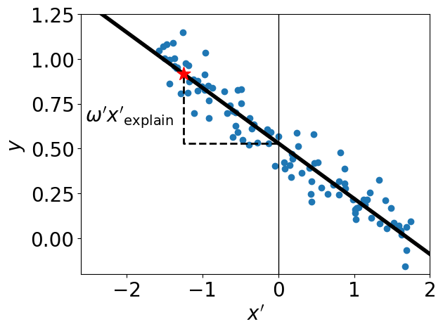
This new model \(h’\) is essentially a horizontally shifted image of the original one \(h\). Although it is not the same function, they make the same prediction on the data. That is, the individual \(x_{\text{explain}}’\) (the red star) is still predicted as high risk and so their loan is rejected. Using this new model, the explanation \(\omega_1’x’_{\text{explain}}\) becomes

print(f"Local Importance of x_explain_prime : {float(model_prime.coef_[0]*x_explain_prime[0]):.2f}")
>> Local Importance of x_explain_prime : 0.39

This is not the same feature importance that we had for \(h(x_{\text{explain}})\) (it was -1.15). This is problematic because the loan applicant can receive two different explanations for the same loan rejection.

Feature Importance scores should be invariant to modeling choices that keep the predictions on data intact. Such choices include any affine transformation \(x’=ax+b\) applied before training a Linear Model.

Correctly Explaining Linear Models

We just saw that the naive local feature importance \(\omega_i x_i\) is not invariant to affine transformations of the input feature \(i\). The solution to solve this issue is to think local feature importance as being relative and not absolute. That is, instead of explaining the prediction \(h(x)\), one should answer a contrastive question of the form : why is the model prediction \(h(x)\) so high/low compared to a baseline value? The baseline value is commonly chosen to be the average output \(\mathbb{E}_{z\sim\mathcal{B}}[h(z)]\) over a probability distribution \(\mathcal{B}\) called the background. At the heart of any contrastive question is a quantity called the Gap

which is the difference between the prediction of interest \(h(x)\) and the baseline. Examples of contrastive questions include:

1. Why is individual \(x\) predicted to have higher-than-average risks of heart disease? Here, the Gap is positive and the background \(\mathcal{B}\) is the distribution over the whole data.
2. Why is house \(x\) predicted to have a lower price than house \(z\)?. In that case, the Gap is negative and the background \(\mathcal{B}\) is the Dirac measure \(\delta_z\) centered at house \(z\).

Here is how the package PyFD advocates reporting the local importance of \(x_i\) toward the Gap.

These local importance measure have the property of summing to the Gap

but are they are also invariant to affine transformations (\(x’=ax+b\)) on individual input features. To see how, lets go back to our toy model and answer the question : why is the red star individual predicted a higher default risk than the average population? To answer this contrastive question, we must set the background distribution \(\mathcal{B}\) to the empirical distribution over the whole dataset.

from pyfd.decompositions import get_components_linear
from pyfd.feature import Features

# We have a single numerical feature
features = Features(X, ["x"], ["num"])

### Original data
# Foreground is the point to explain
foreground = x_explain.reshape((1, -1))
# Background is the distribution over the whole data
background = X
# Under the hood, PyFD returns : Importance x_i = omega_i (x_i - E[z_i])
decomposition = get_components_linear(model, foreground, background, features)
print(f"Local Importance of x_explain : {decomposition[(0,)][0]:.2f}")
>> Local Importance of x_explain : 0.39

### Standardized data
# Foreground is the point to explain
foreground = x_explain_prime.reshape((1, -1))
# Background is the distribution over the whole data
background = X_prime
# Under the hood, PyFD returns : Importance x_i' = omega_i' (x_i' - E[z_i'])
decomposition = get_components_linear(model_prime, foreground, background, features)
print(f"Local Importance of x_explain_prime : {decomposition[(0,)][0]:.2f}")
>> Local Importance of x_explain_prime : 0.39

As we can see, the local importance of feature \(x\) is the same regardless of whether we standardize the input feature or not. Consequently, the explanation for the loan rejection of the applicant (the red star) could be phrased as

The feature x (maybe salary which is lower than average) explains 0.39 of your increase in risks relative to the average population.

Ouverture

I hope you can appreciate that explaining a Linear Model is not as trivial is it might seem at first glance. The notion of explaining predictions \(h(x)\) relative to the average prediction \(\mathbb{E}_{z\sim\mathcal{B}}[h(z)]\) over a background distribution \(\mathcal{B}\) appears naturally when we wish to derive Linear Model explanations that are invariant to modeling choices such as feature standardization. In future blogs, we will see that relative explanations also appear naturally when investigation a more general class of models : Additive Models.