Explaining Parametric Additive Models

In this third blog post, we discuss Parametric Additive Models, which are simply Linear Models applied on univariate basis functions rather than the original features. Like with Linear Models, viewing local explainability as a relative concept (explaining a prediction relative to a baseline) is necessary to get rid of mathematical inconsistencies.

Additive Models

Additive Models are functions that take the following form

where the shape function \(h_i\) only depends on a single feature \(x_i\). Note that linear models are a special case of additive models with \(h_i(x_i) = \omega_i x_i\). Additive Models are considered interpretable for the following reasons.

1. The effect of varying feature \(x_i\) on the response \(h(x)\) is independent of the fixed values of the remaining features \(x_1, \ldots, x_{i-1}, x_{i+1}, \ldots, x_d\).
2. The effect of varying feature \(x_i\) on the response \(h(x)\) is entirely encoded in the corresponding shape function \(h_i\).

These properties imply that one only needs to visualize the shape function \(h_i\) to understand how varying feature \(x_i\) affects the model output. Moreover, all shape functions can be visualized simultaneously to get an overview of the model \(h\).

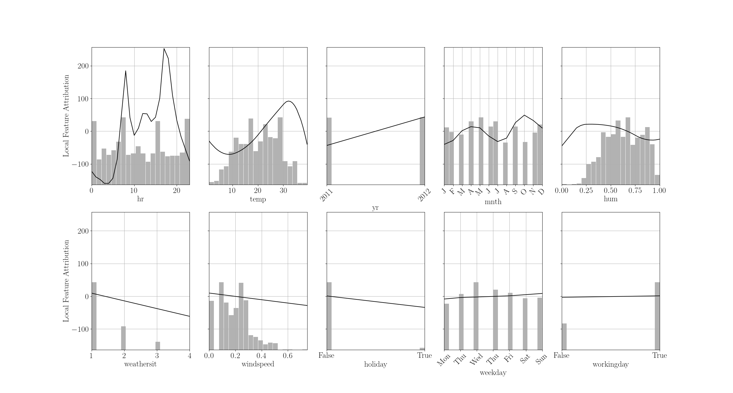
This is an example of additive model trained to predict of number of bike rentals given time and weather features. By looking at all shape functions in tandem, you can see how the model reasons.

Additive Models are the second floor of the ladder we must climb before being able to explain general black-boxes.

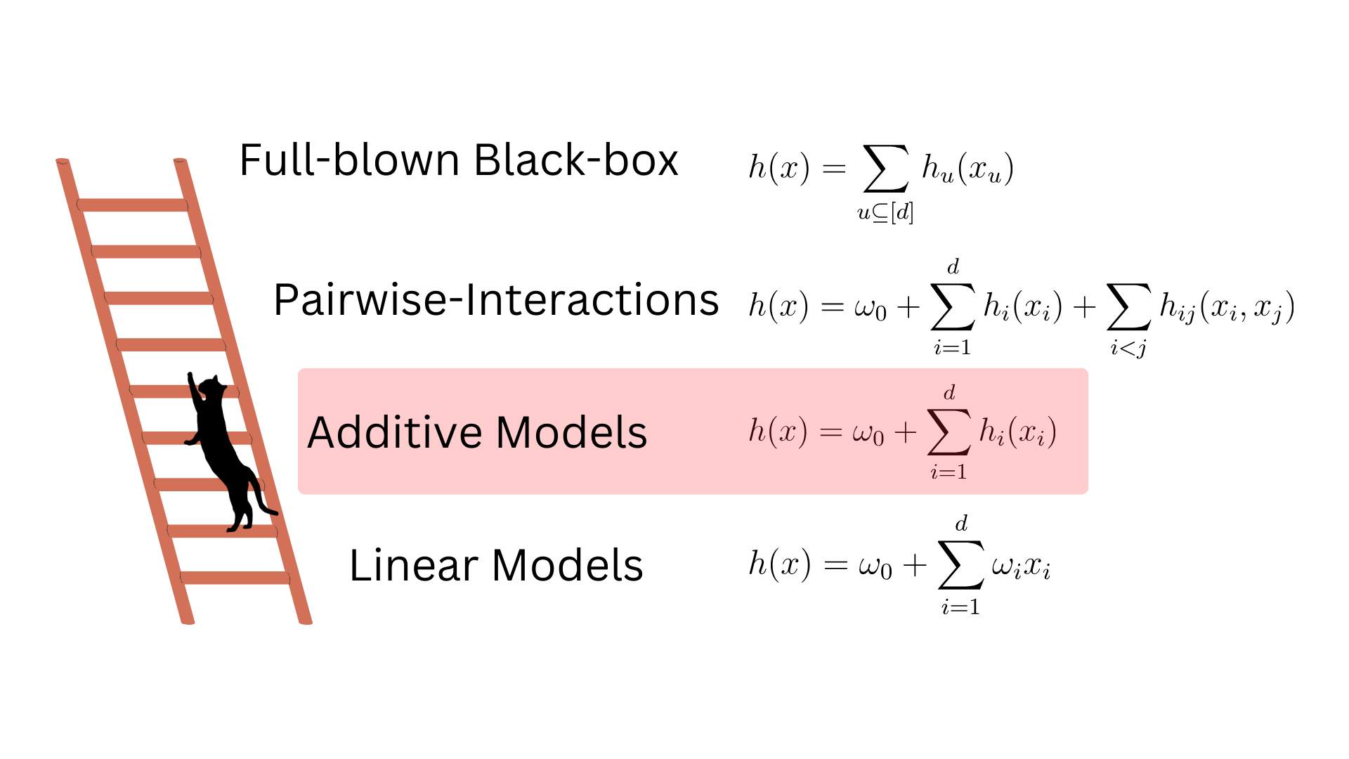
Such models are more complex than Linear ones because the shape functions \(h_i\) can potentially be highly non-linear. But they are still more interpretable than general black-boxes because we understand how individual input features impact the model response.

Parametric Additive Models

We shall introduce Additive Models on a toy example with two features \(x_1,x_2\sim U(0, 1)\) and with a target \(y = x_1^2 + \cos(2\pi x_2)+\epsilon\), where \(\epsilon\) is random Gaussian noise.

import numpy as np
import matplotlib.pyplot as plt
np.random.seed(42)
from pyfd.features import Features

# Two input features
X = np.random.uniform(0, 1, size=(200, 2))
# Feature object
features = Features(X, ["x1", "x2"], ["num", "num"])
# The label is an additive function
y = X[:, 0]**2 + np.cos(2*np.pi*X[:, 1]) + 0.1 * np.random.normal(size=(200,))

Since the target is an additive function of the input features, we should be able to accurately approximate it with an additive model. Now, fitting additive models requires defining a representation of the shape functions \(h_i\). We cannot allow any possible function since this would render the training intractable. There are two solutions : Parametric and non-parametric representations. In this blog, we will investigate Parametric Additive Models, and the subsequent blog-post will illustrate the alternative.

In a parametric model, each shape function \(h_i\) is modelled by first defining a basis of \(M_i\) functions along each feature \(i\) : \(h_{i1}(x_i), h_{i2}(x_i),\ldots h_{iM_i}(x_i)\). For shape functions \(h_i\) that are piece-wise linear, we define a basis of piece-wise linear functions along feature \(x_i\).

from sklearn.pipeline import Pipeline
from sklearn.preprocessing import SplineTransformer, FunctionTransformer

# degree=1 spline basis
n_knots = 5
splines = SplineTransformer(n_knots=n_knots, degree=1).fit(X)

# Plot the basis functions h_{11}, h_{12}, ..., h_{1M_1} over the whole x_1 axis
plt.figure()
line = np.linspace(0, 1, 200)
H_line = splines.transform(np.column_stack((line, line)))
plt.plot(line, H_line[:, :n_knots], linewidth=4)
plt.xlabel("x1")
plt.ylabel("Spline Basis")
knots = splines.bsplines_[0].t
plt.vlines(knots[1:-1], ymin=0, ymax=1.05, linestyles="dashed", color="k")
plt.ylim(0, 1.1)

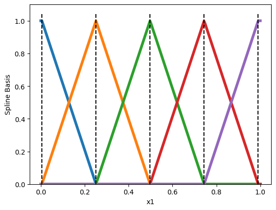
Each pyramid is a single basis function \(h_{ij}(x_i)\). Then, we express the shape function \(h_i\) as a linear combination of these basis functions

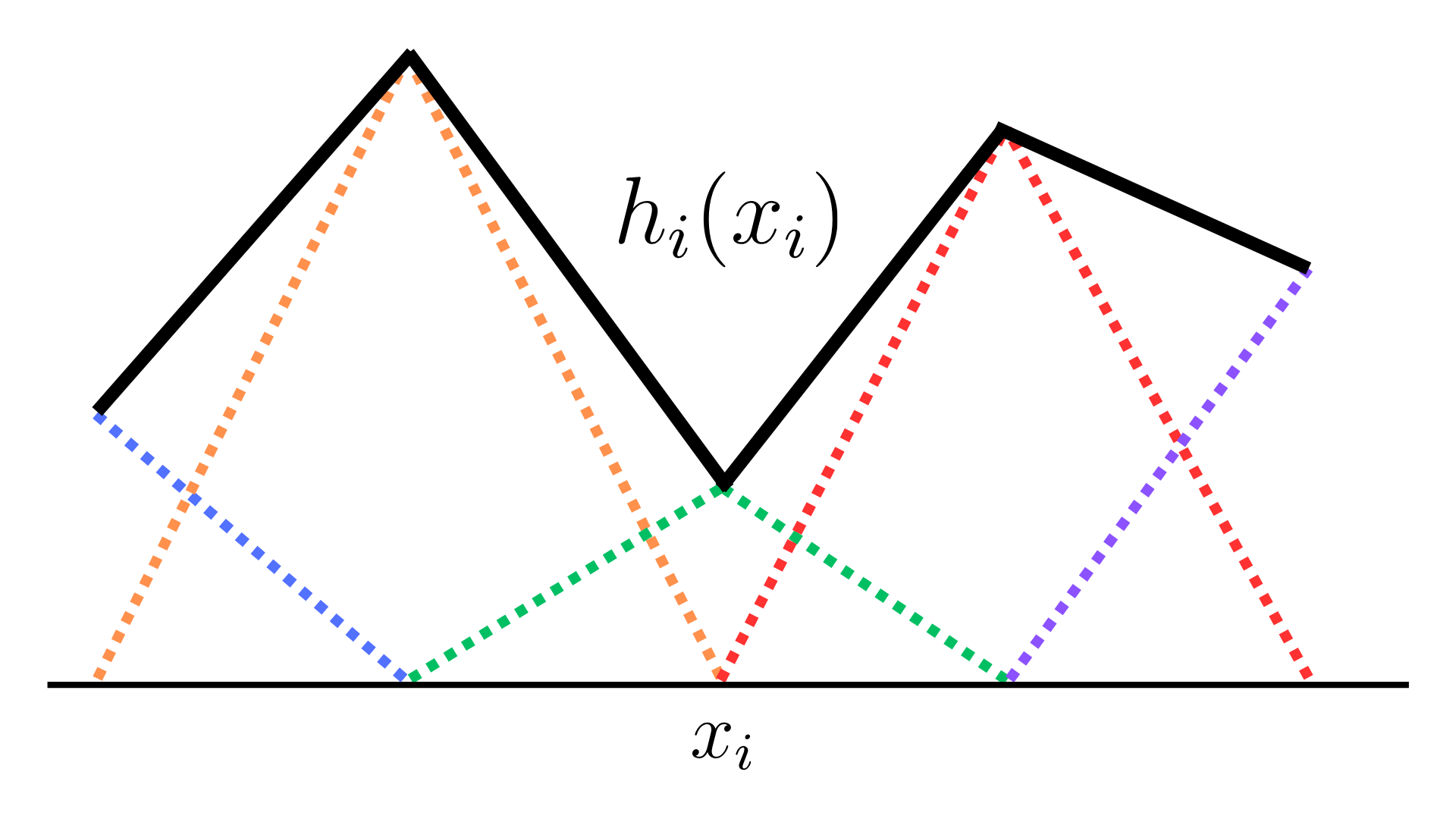
Repeating this procedure for all features leads to the following additive model

This model is nothing more than a Linear Model applied on the \(N\times \sum_{i=1}^d M_i\) augmented matrix H (containing the basis function evaluations over all data) instead of the raw inputs \(N\times d\) matrix X. Fitting a LinearRegression using H leads to a model with a low error.

from sklearn.linear_model import LinearRegression

# A (N, 10) matrix of all splines evaluated on all data points
H = splines.transform(X)

# Linear Model with poor performance
linear_model = LinearRegression().fit(X, y)
print(linear_model.score(X, y))
>> 0.13

# Additive Model with great performance
parametric_additive_model = LinearRegression().fit(H, y)
print(parametric_additive_model.score(H, y))
>> 0.97

Naively Explaining Parametric Additive Models

Given that the output of an additive model is the summation of all shape functions and the intercept \(\omega_0\), it is tempting to define the following local importance of feature \(x_i\) toward a given prediction \(h(x)\).

However, we saw that the analogous definition for linear models (\(\text{Local Importance of } x_i = \omega_i x_i\)) was problematic, and so this definition cannot be right. To see why this definition is incorrect, note that basis functions are redundant with the intercept \(\omega_0\). Indeed, the basis functions presented previously sum up to one at any \(x_i\)

So any vertical shift in prediction \(h(x) + C\) could be accomplished by either adding \(C\) to the intercept \(\omega_0\), or by adding \(C\) to all weights : \(\omega_{i1}, \omega_{i2}, \ldots \omega_{iM_i}\). Consequently, there is an infinite number of weights \(\omega\) that fit the data well. The Scikit-Learn class LinearRegression was kind enough to return a single solution (using a pseudo-inverse), but don’t be fooled: there is an infinity of solutions.

Adding the same constant \(C\) to all weights \(\omega_{i1}, \omega_{i2}, \ldots \omega_{iM_i}\) and removing \(C\) from the intercept \(\omega_0\) leads to an identical function \(h’\) but with different local feature importance.

The typical methodology to yield a single optimal solution \(\omega\) is to remove one basis function along each feature \(i\). This will ensure that the basis functions do not sum to \(1\) and so they are no longer redundant with the intercept.

# Passing `include_bias=False will remove on basis along each feature
n_knots = 10
splines = SplineTransformer(n_knots=n_knots, degree=1, include_bias=False).fit(X)

# Plot the basis functions on the whole x axis
plt.figure()
line = np.linspace(0, 1, 200)
H_line = splines.transform(np.column_stack((line, line)))
plt.plot(line, H_line[:, :n_knots-1], linewidth=4)
plt.xlabel("x1")
plt.ylabel("Reduced Spline Basis")
knots = splines.bsplines_[0].t
plt.vlines(knots[1:-1], ymin=0, ymax=1.05, linestyles="dashed", color="k")
plt.ylim(0, 1.1)

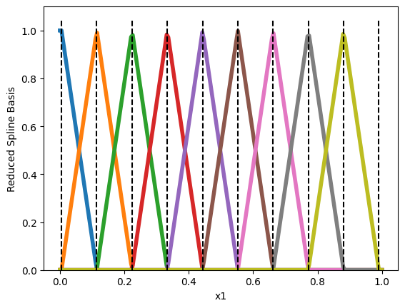
By default, Scikit-Learn removes the last basis function. This guarantees that a single optimal \(\omega\) exists. Yet, by removing the last basis, we inevitably attribute no importance to feature \(x_i\) whenever it is equal to \(1\). This is because all basis functions are null when \(x_i=1\) and so \(h_i(1) = \sum_{j=1}^{M_i}\omega_{ij} 0 = 0\). This choice is arbitrary and we might as well remove the first basis function (which can be done with the following hack).

# Flipping the feature before feeding it to `SplineTransformer` is a hack to
# remove the first basis function.
splines_reversed = Pipeline([('reverse', FunctionTransformer(lambda x: -x)),
                             ('splines', SplineTransformer(n_knots=n_knots, degree=1, include_bias=False))
                            ]).fit(X)

# Plot the basis functions on the whole x axis
plt.figure()
line = np.linspace(0, 1, 200)
H_line = splines_reversed.transform(np.column_stack((line, line)))
plt.plot(line, H_line[:, n_knots-1::-1], linewidth=4)
plt.xlabel("x1")
plt.ylabel("Reduced Spline Basis")
knots = -1 * splines_reversed.steps[1][1].bsplines_[0].t
plt.vlines(knots[1:-1], ymin=0, ymax=1.05, linestyles="dashed", color="k")
plt.ylim(0, 1.1)

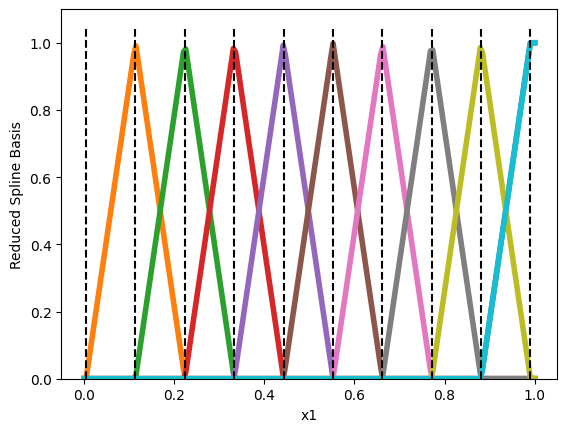
In that scenario, the first basis function is removed and so feature \(x_i\) will get no importance whenever it is equal to \(0\).

Although removing a basis function ensures that a single optimal weight vector \(\omega\) exists, the choice of which basis to remove is arbitrary and leads to ambiguous local feature importance.

Correctly Explaining Linear Models

The naive local feature importance \(h_i(x_i)\) is not invariant to the choice of which basis function to remove. Like previously with Linear Models, the solution to render explanations invariant is to think local feature importance as being relative and not absolute. That is, instead of explaining the prediction \(h(x)\), one should answer a contrastive question of the form : why is the model prediction \(h(x)\) so high/low compared to a baseline value? The baseline value is commonly chosen to be the average output \(\mathbb{E}_{z\sim\mathcal{B}}[h(z)]\) over a probability distribution \(\mathcal{B}\) called the background. At the heart of any contrastive question is a quantity called the Gap

which is the difference between the prediction of interest \(h(x)\) and the baseline.

Here is how the package PyFD advocates reporting the local importance of \(x_i\) toward the Gap.

These local importance measure have the property of summing to the Gap

but are they are also invariant to the choice of which basis function is removed. To confirm, we compute two additive models that either remove the last or the first basis. By comparing their predictions over the whole data, we confirm both models are indeed different parametrizations of the same function.

# We remove the last basis function
additive_model_1 = Pipeline([('splines', SplineTransformer(n_knots=n_knots, degree=1, include_bias=False)),
                             ('predictor', LinearRegression())
                            ]).fit(X, y)
# We remove the first basis function
additive_model_2 = Pipeline([('reverse', FunctionTransformer(lambda x: -x)),
                             ('splines', SplineTransformer(n_knots=n_knots, degree=1, include_bias=False)),
                             ('predictor', LinearRegression())
                            ]).fit(X, y)

# The models are two different parametrization of the same function
assert np.isclose(additive_model_1.predict(X), additive_model_2.predict(X)).all()
>> True

To compute the local feature importance using PyFD, we employ the function get_components_linear, which was used in the previous blog post about Linear Models. Indeed, since Parametric Additive Models are just Linear Models applied on basis functions rather than raw data, the function get_components_linear is still applicable. PyFD is intelligent enough to notice that the Linear Model is applied over basis functions and will compute the correct local feature importance.

from pyfd.decompositions import get_components_linear
from pyfd.plots import partial_dependence_plot

# We explain the predictions on all data points
foreground = X
# The baseline is the average prediction over the data
background = X
# Under the hood, PyFD computes importance x_i = h_i(x_i) - E[ h_i(z_i) ]
# with h_i(x_i) = sum_{j=1}^{M_i} omega_{ij} h_{ij}(x_i)
decomposition_1 = get_components_linear(additive_model_1, foreground, background, features)
decomposition_2 = get_components_linear(additive_model_2, foreground, background, features)

# Local Feature Importance of the first model
partial_dependence_plot(decomposition_1, foreground, background, features, plot_hist=True)

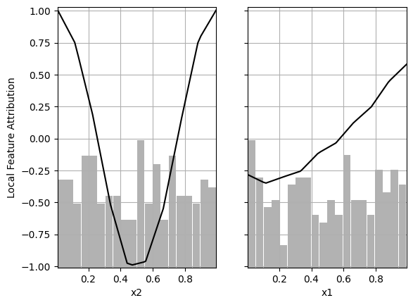
# Local Feature Importance of the second model
partial_dependence_plot(decomposition_2, foreground, background features, plot_hist=True)

As we can see, the local feature attribution is the same regardless of which basis function is removed.

Ouverture

To resume, we introduced Additive Models, which are interpretable because the effect of varying feature \(x_i\) is entirely encoded in the shape function \(h_i(x_i)\). Nonetheless, explaining individual predictions \(h(x)\) of said models is not trivial because the shape functions \(h_i(x_i)\) are redundant with the inclusion of an intercept \(\omega_0\) within the model. Viewing local explainability as a relative concept gets rid of this ambiguity.