Explaining Non-Parametric Additive Models

This fourth blog post discusses Non-Parametric Additive Models, and more specifically Explainable Boosting Machines (EBMs for short). EBMs are state-of-the-art interpretable models invented by Rich Caruana from Microsoft Research. We will see how these models provide built-in explanations for their decisions, how they can be edited to be more intuitive, and how they can explain disparities between demographic subgroups.

Additive Models

Additive Models are functions that take the following form

We have seen previously how to model the shape functions using basis function multiplied by learned parameters. The issue with this method is that the basis functions must be determined apriori. How many basis functions should be used? Where should they be placed? Bad basis placemement may lead to subpar performance, especially if there are steep jumps in the function that must be approximated. Fitting such jumps would require placing sufficiently many basis functions at the correct position before even fitting the model.

The alternative is to not employ parameters and instead use Univariate Decision-Trees to represent the shape function \(h_i\). A Univariate Decision Tree \(t(x_i)\) is a tree whose internal nodes encode boolean statements (True or False) on feature \(x_i\), and whose leaf encode a single prediction.

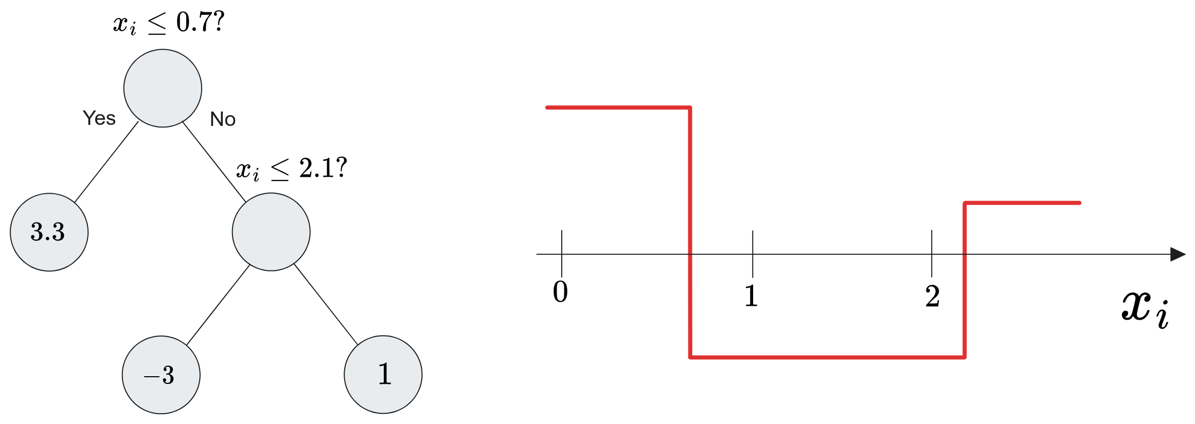
To extract predictions from a decision tree, you start from the root and follow the edges downward going in the direction indicated by the boolean statement. Once you reach a leaf, the prediction is given by its value.

Decision trees are more flexible than splines basis functions because the placement of their jumps are adapted to the data and are not fixed beforehand. Moreover, decision trees can model very steep jumps since (unlike splines) they are discontinuous functions. Nevertheless, trees are prone to overfitting the data because of their high flexibility and it is common to train an ensemble of decision tree to smooth them out.

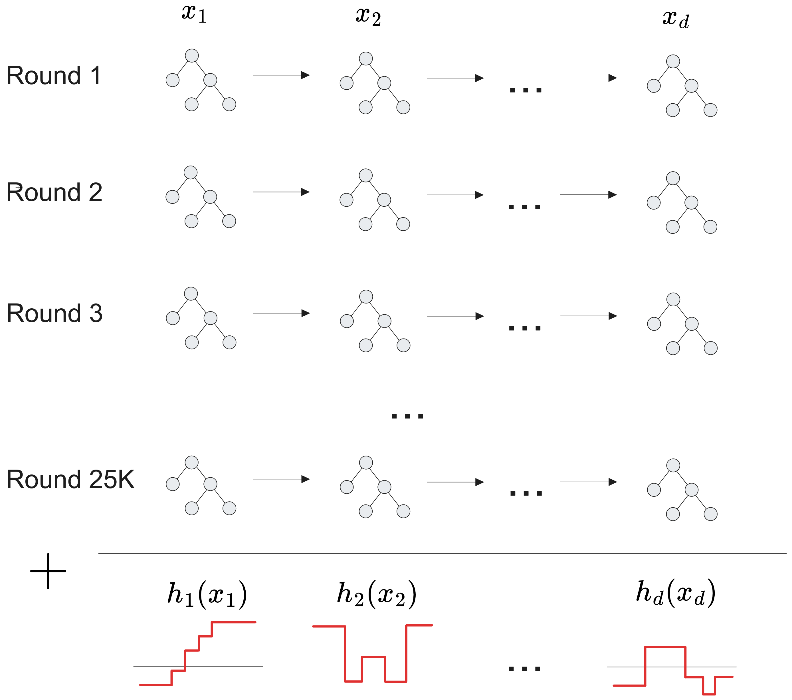
The idea behind ExplainableBoostingMachines (EBMs for short) from the Interpret Python Library is to learn an ensemble of Univariate Decision Trees \(t_1,t_2,\ldots, t_{25000\times d}\) in a round-robin fashion (fit \(t_1\) on \(x_1\), fit \(t_2\) on \(x_2\), …, fit \(t_d\) on \(x_d\), fit \(t_{d+1}\) on \(x_1\) etc.). Each tree \(t_k\) is trained to minimize the error made by all previous trees. After many rounds, all trees involving feature \(x_i\) are summed, yielding the shape function

This procedure is illustrated as follows.

Income Prediction

Fitting the Model

The Adult-Income dataset aims at predicting whether individuals in the US make more (\(y=1\)) or less (\(y=0\)) than 50K USD. The data contains 49K instances taken from the 1994 Census. Although this dataset is outdated, it is still popular as a baseline for new ideas in the explainability and fairness fields. The PyFD implementation of this dataset is used.

from pyfd.data import get_data_adults

X, y, features, gender = get_data_adults(remove_gender=True)
print(X.shape)
>> (48842, 11)
print(y[:20])
>>[0 0 0 0 0 0 0 0 0 0 1 1 0 0 0 0 0 1 0 0]
print(gender[:10])
>>['Male', 'Female', 'Male', 'Female', 'Male', 'Male', 'Male', 'Male', 'Female', 'Female']
features.summary()
|Idx|        Name        |        Type        |    Card    |      Groups      |
-------------------------------------------------------------------------------
| 0 | age                | num                | inf        | [0]              |
| 1 | educational-num    | num                | inf        | [1]              |
| 2 | capital-gain       | sparse_num         | inf        | [2]              |
| 3 | capital-loss       | sparse_num         | inf        | [3]              |
| 4 | hours-per-week     | num                | inf        | [4]              |
| 5 | workclass          | nominal            | 4          | [5]              |
| 6 | education          | nominal            | 8          | [6]              |
| 7 | marital-status     | nominal            | 5          | [7]              |
| 8 | occupation         | nominal            | 6          | [8]              |
| 9 | relationship       | nominal            | 6          | [9]              |
| 10| race               | nominal            | 5          | [10]             |
-------------------------------------------------------------------------------``

Adult-Income involves 11 features and a binary target so it is called a classification task. It also contains a gender features that takes values Female and Male. Depending on your use-case, you might be prohibited by law from using this feature for predictions. So, we removed it from the matrix X. Consequently, the model cannot have direct access to its value. The values for gender are kept in a separate array.

Here is how an EBM can be trained to make accurate predictions of income category.

from sklearn.model_selection import train_test_split
from interpret.glassbox import ExplainableBoostingClassifier
# Split the data in to train and test sets.
X_train, X_test, y_train, y_test, gender_train, gender_test = train_test_split(X, y, gender,
                                                                               test_size=0.3, 
                                                                               stratify=y, 
                                                                               random_state=42)
# Fit model with default hyperparameters
model = ExplainableBoostingClassifier(random_state=0, interactions=0, n_jobs=-1)
model.fit(X_train, y_train)

Now, to evaluate this model we must choose a performance metric : the simplest one in classification being the accuracy

where \(1(\cdot)\) is an indicator function, \(\widehat{y}^{(i)}\) is the binary prediction at instance \(x^{(i)}\) and \(y^{(i)}\) is the actual label. Accuracy is simply the ratio of samples on which the model makes the correct binary decision. Importantly, since EBMs return a numerical score (e.g. \(h(x^{(i)})=2.537\)), a cutoff treshold \(\gamma\) must be used to yield a binary decision :

The default value of the threshold is \(\gamma=0\) but note that it can be tuned for your specific use-case and performance metrics. We return the test set accuracy of the EBM using its .score method.

print(model.score(X_test, y_test))
>>> 0.868

Naively Explaining the Model

Now that we have fitted the EBM, we wish to understand its predictions in order to validate them. The following definition of local importance for feature \(x_i\) is very tempting

However, this formulation has a key problem : the non-parametric shape functions \(h_i\) could be modified by adding a constant \(C\) to all leaves of the decision trees involving \(x_i\). This vertical shift in \(h_i\) could be cancelled out by adjusting the intercept \(\omega_0\) accordingly

Although \(h\) and \(h’\) make identical predictions on any input, the local importance they attribute to \(x_i\) can vary arbitrarily.

Adding a constant \(C\) to the non-parametric shape function \(h_i\) and removing this constant from the intercept \(\omega_0\) leads to an identical function \(h’\) but with different local feature importance.

Correctly Explaining the Model

Rather than explaining the prediction \(h(x)\), we should explain the Gap between the prediction and a reference.

PyFD advocates reporting the local importance of a feature as follows

These local importance scores satisfy the crucial property of summing up to the Gap

so they can be seen as explaining the Gap. Moreover, these quantities are invariant to the choice of constant \(C\) that we add to the shape functions. PyFD provides built-in functions to compute the local feature importance of an EBM model.

from pyfd.decompositions import get_components_ebm
from pyfd.plots import partial_dependence_plot

# The reference data
background = X
# We want to explain the predictions at each test instance
foreground = X_test
# Under the hood, PyFD computes : Imp x_i = h_i(x_i) - E_{z~B}[h_i(z_i)] 
decomp = get_components_ebm(model, foreground, background, features)
# Plot the local feature importance
partial_dependence_plot(decomp, foreground, features)

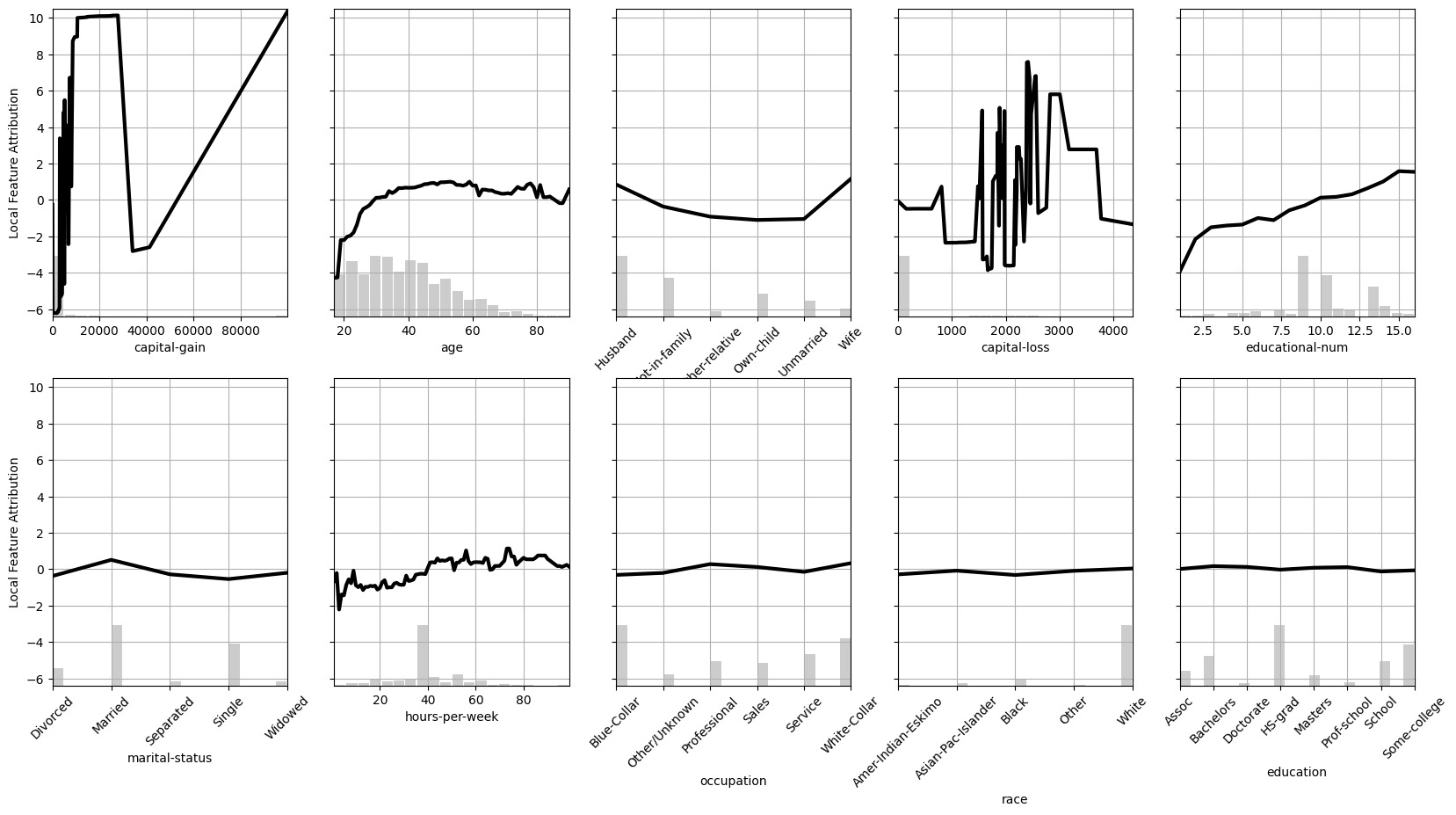
This plot reveals some insight on the EBM.

• The EBM has learned that the likelihood of making money increases with age and educational-num.
• Being a Husband or Wife increases the likelihood as well according to the model.
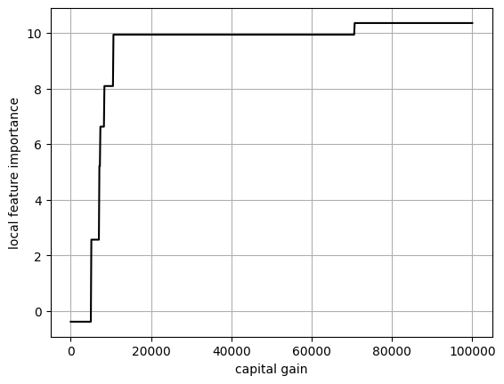
• Larger capital-gain is associated with greater chances of making more than 50K, except for a weird drop near 40K.

The large drop in local importance for capital-gain is very peculiar so we investigate it further.

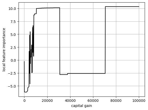
We see that the drop in local importance occurs in the 30K-70K range. Intuitively, the likelihood of making money should increase with captical-gain so this behavior is really unexpected. I suspect that this is due to noise in the data : perhaps some individual within this range had typos in their target. Or maybe there is an unknown confounding variable that explains this drop. Either way, we cannot know for sure since this dataset is so old.

One of the advantages of EBMs is that their shape functions can be corrected to better fit with prior knowledge about a task. Here, we can enforce a monotonous relationship between capital gain and income.

# This will modify the model in-place.
model.monotonize(feature_idx)
# The test-accuracy will be slightly reduced
print(model.score(X_test, y_test))
>> 0.863

The fun part is that model editing is cheap in terms of computations and can be done after the model is trained. There is no need to retrain from scratch.

Explaining Disparities

Fairness is a growing topic in Machine Learning because, although models hold the promise of providing objective opinions based on empirical data, their strong reliance on historical data means that they can perpetuate past injustices/discrimination. In the case of the Adult-Income dataset, in 1994 there was an imbalance in income between men and women, which is inherited by the learned model. We can report the Gap

to see a difference favoring men.

We are reporting Gaps in the numerical score \(h(x)\) and not the binary predictions \(\widehat{y}\). Although it is more common in the literature to report disparities in binary predictions, such reports have the downsides of depending on the choice of cuttoff treshold \(\gamma\) and not being additive. Disparities in the numerical outputs \(h(x)\), on the other hand, are not affected by \(\gamma\) and are explainable by design.

# Use the gender feature to partion the test set in to women and men
test_women = X_test[gender_test=="Female"]
test_men = X_test[gender_test=="Male"]
# model.decision_function returns the numerical output
Gap = model.decision_function(test_men).mean() - model.decision_function(test_women).mean()
print(Gap)
>> 1.95

On average, men have an output that is higher than women by almost 2. What are the causes of this disparity? Remember that the gender feature is not accessible by the model. As a result, this is a case of indirect discrimination, which can be legal depending on which factors (or proxies) are inducing the disparity.

Think for instance of firefighting departments. Their gender imbalance can be explained by the strong physical requirements and correlations between strength and sex due to biological nature. Therefore, as long as a firefighting department is solely relying on strength criteria to select employees, it is unlikely to be sued for gender discrimination.

The same applies for our predictive model. We would like the factors inducing a difference between men and women to be meritocratic and not arbitrary. PyFD reports the following importance of \(x_i\) toward the men-women disparity

These importance scores sum to the Gap between men and women.

from pyfd.plots import bar

# Compute the local feature importance for all men and women
decomp_women = get_components_ebm(model, test_women, background, features)
decomp_men = get_components_ebm(model, test_men, background, features)
# Compute E[h_i(x_i)|man] - E[h_i(x_i)|woman] 
fairness_importance = np.stack([decomp_men[(i,)].mean() - decomp_women[(i,)].mean() for i in range(len(features))])
bar(fairness_importance, features.names())

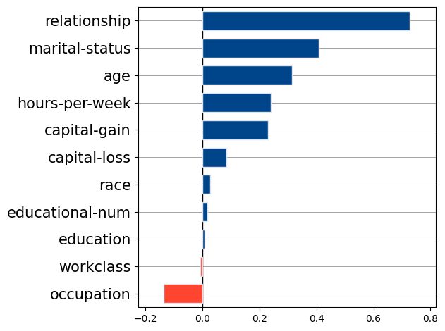
The main factors favoring men are relationship, marital-status, age, capital-gain, and hours-per-week. We can visualize how the features relationship and marital-status induce a disparity.

from pyfd.plots import plot_legend

partial_dependence_plot([decomp_men, decomp_women], [test_men, test_women], features, idxs=[7, 9]))
plot_legend(["Men", "Women"])

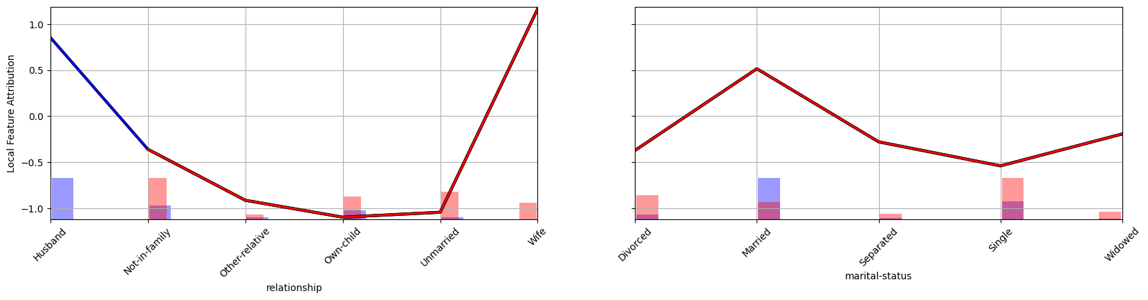
The blue distribution represents men, while in red one represents women. The importance of \(x_i\) toward the men-women Gap is the difference between the average of \(h_i\) for the blue and red distributions. These plots reveal that a larger proportion of women (compared to men) are not married. Since being married increases the model numerical output, men have (on average) a higher score than women.

Ouverture

Explainable Boosting Machines (EBMs) are state-of-the-art Non-Parametric Additive Models. Such models can be explained locally, they can be edited to better align with prior-knowledge, and they can explain disparities between subgroups (e.g. men and women). As a result, EBMs are my go-to method whenever I am starting a new Machine Learning project.