The Disagreement Problem in Explainability

In this first blog post, we will discuss post-hoc explanation methods and whether they are just another black-box on top of the Machine Learning model.

Machine Learning Models

Machine Learning aims at teaching computers how to solve complex problems. This methodology is useful for solving tasks where it is hard to write a conventional program. For example, lets say you are working for a bike rental company and you want to predict the number of bike rentals at a certain hour given information about the weather and the day of the week. A classical program might look like this

if temperature=cold or time=late or time=early:
  return few-bike-rentals
else if temperature=hot_but_not_too_hot:
    return many-bike-rentals
else:
  return medium-bike-rentals

This program has several issues. First, it is not clear what hot and cold temperature actually mean numerically. What thresholds should be used? Same thing with time=late and time=early. The solution proposed with Machine Learning is to learn those thresholds (and the program itself) automatically based on historical data of bike rentals given various hours and temperatures. In this new paradigm, you would need access to data comprised of

1. A \((N, d)\) feature matrix X representing the \(d\) characteristics (time, temperature, day of the week etc.) of \(N\) instances.
2. A \((N,)\) vector y containing the actual number of bike rentals for the given instance.

Here is an example of such a dataset available in the package PyFD .

import numpy as np
import matplotlib.pyplot as plt
from pyfd.data import get_data_bike

# load the data
X, y, features = get_data_bike()
print(X.shape)
>>> (17379, 10)
print(y.shape)
>>> (17379,)
print(features.names())
>>> ['yr', 'mnth', 'hr', 'holiday', 'weekday', 'workingday', 'weathersit', 'temp', 'hum', 'windspeed']

We have 17K data instances each comprised of \(d=10\) time/weather features. Given this collection of data, one then fits a Machine Learning model \(h\) in order to get accurate predictions of \(y\) given \(x\). In this blog, we will investigate three regressors:

1. Random Forests
2. Gradient Boosted Trees
3. Neural Networks.

To assert if these models are good or not, we have to keep aside some portion of the data (here 20%) and used it afterward to compute an unbiased measure of performance. The \(R^2\) measure of performance is used

where \(\bar{y}\) is the average value of the target on the test set. Simply put, the \(R^2\) represents how better the model \(h\) is at predicting \(y\) than the dummy predictor \(h^{\text{dummy}}=\bar{y}\).

from sklearn.pipeline import Pipeline
from sklearn.preprocessing import StandardScaler
from sklearn.neural_network import MLPRegressor
from sklearn.ensemble import RandomForestRegressor, HistGradientBoostingRegressor
from sklearn.model_selection import train_test_split

# Split the data
X_train, X_test, y_train, y_test = train_test_split(X, y, test_size=0.2, random_state=42)

# Fit the models
model_1 = Pipeline([('preprocessor', StandardScaler()), 
                    ('predictor', MLPRegressor(random_state=0, 
                                               max_iter=1000,
                                               learning_rate_init=0.01))]).fit(X_train, y_train)
model_2 = RandomForestRegressor(random_state=0, max_depth=10).fit(X_train, y_train)
model_3 = HistGradientBoostingRegressor(random_state=0).fit(X_train, y_train)

# Evaluate the models
print(f"R^2 of model_1 : {model_1.score(X_test, y_test):.3f}")
print(f"R^2 of model_2 : {model_2.score(X_test, y_test):.3f}")
print(f"R^2 of model_3 : {model_3.score(X_test, y_test):.3f}")

>>>
R^2 of model_1 : 0.908
R^2 of model_2 : 0.919
R^2 of model_3 : 0.943

Note that the three models have acceptable performance on the test set and hence these programs are able to accurately predict the number of bike rentals.

Post-hoc explanations

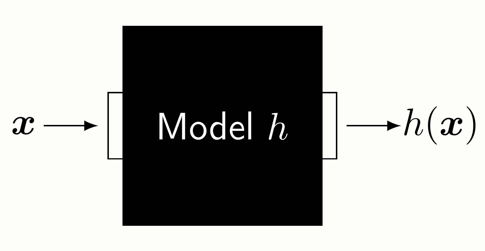
Let’s be frank, do you think that the three models presented earlier are trustworthy? Would you deploy them if you were working at a bike rental company? Personally, the current results are not enough to convince me. Indeed, we have reported some encouraging indices of performance, yet we do not know how the program works internally. What if there is a bug in the model? What if the model does not work well in deployment? We cannot answer those questions with certainty because our models are black-boxes: they take an input \(x\) and return an output \(h(x)\), but we do not understand the mechanisms involved.

Our lack of understanding of \(h\) is the main motivation behind eXplainable Artificial Intelligence (XAI), a research initiative to shed light on the decision-making of ML models. This research field has recently introduced many techniques

1. Local Feature Attributions \(\phi_i(h, x)\,\forall i=1,2,\ldots,d\) are vectors that attribute to each feature an importance toward the prediction \(h(x)\).
2. Global Feature Importance \(\Phi_i(h)\,\forall i=1,2,\ldots,d\) are positive vectors that illustrates how much the feature is used overall by the model.

We will focus on Global Feature Importance as they are the simplest to understand. We will employ three techniques Partial Dependence Plots (PDP), Permutation Feature Importance (PFI), SHAP. Here is how you would compute them on model_3.

from pyfd.decompositions import get_components_tree, get_PDP_PFI_importance
from pyfd.shapley import interventional_treeshap, get_SHAP_importance
from pyfd.plots import bar

decomposition = get_components_tree(model_3, X_test, X_test, features, anchored=True)
shapley_values = interventional_treeshap(model_3, X_test, X_test, features, algorithm="leaf")
I_PDP, I_PFI = get_PDP_PFI_importance(decomposition)
I_SHAP = get_SHAP_importance(shapley_values)
bar([I_PFI, I_SHAP, I_PDP], features.names())
plt.xlabel("Global Feature Importance")
plt.show()

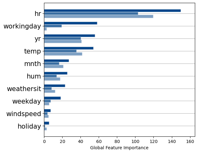
This bar chart presents the feature importance yielded by three different explainers (PFI, SHAP, PDP) in different opacities (opaque, semi-transparent, transparent). We note that all three methods agree the Gradient Boosted Trees rely more on the feature hr than any other features. This is an example of insight that post-hoc explanations can give you on your model.

The Disagreement Problem

However, we see that explainers do not agree on the importance of workingday : PFI says its the second most important feature while PDP says it is not important at all. Which one of these interpretations is correct? This is an important question to address because if we cannot trust the post-hoc explainers, we cannot trust the model in the first place and we are back to square one.

The simple example of explanation disagreements I presented occurs in a variety of ML use-cases and models. Even worse, (Krishna et al., 2022) have interviewed 25 data scientists who use XAI techniques daily and found out that they did not know how to handle disagreements between explainability methods. Practitionners instead relied on heuristics such as sticking to their prefered method or whichever explanations best matched their intuition.

Still, we argue that choosing explanations this way is risky since humans are prone to confirmation biases. It is better to select the correct explanation based on their correctness, which leads to my main research question:

How can the correctness of conflicting post-hoc explanations be determined?

I will not have the time to present my ideas/solutions in this blog post, but future posts will discuss them. Stay tuned!